Published research
ODE Network Model for Nonlinear and Complex Agricultural Nutrient Solution System
2019 · 2019 International Conference on Information and Communication Technology Convergence (ICTC) · 996–1001
Abstract
In closed hydroponic systems, periodic readjustment of nutrient solution is necessary to continuously provide stable environment to plant roots because the interaction between plant and nutrient solution changes the rate of ions in it. The traditional method is to repeat supplying small amount of premade concentrated nutrient solution, measuring total electric conductivity and pH of the tank only. As it cannot control the collapse of ion rates, recent researches try to measure the concentration of individual components to provide insufficient ions only. However, those approaches use titration-like heuristic approaches, which repeat adding small amount of components and measuring ion density a lot of times for a single control input. Both traditional and recent methods are not only time-consuming, but also cannot predict chemical reactions related with control inputs because the nutrient solution is a nonlinear complex system, including many precipitation reactions and complicated interactions. We present a continuous network model of the nutrient solution system, whose reactions are described as differential equations. The model predicts molar concentration of each chemical components and total dissolved solids with low error. This model also can calculate the amount of chemical compounds needed to produce a desired nutrient solution, by reverse calculation from dissolved ion concentrations.
Keywords— nutrient solution, smart farm, system engineering, computational chemistry, simulation, complex system, IoT
I. Introduction
Recently, soilless culture takes center stage in agricultural industry. Closed hydroponic system is one of the most popular hydroponic method because it reduces the cost and hazard of water pollution [1]. As plants continuously absorbs nutrients from the environment, the concentration of individual ions continuously drops. Traditional methods usually measure pH and electrical conductivity (EC) of the nutrient solution to monitor the fertilization status [2-3]. When EC is low, they add premade concentrated solution to the tank and then apply acids to maintain pH.
As the absorption rate of the ions are all different, those approaches gradually destroy the ratio among ions [4] and accumulates excessive ions (sodium, chloride, sulfate and etc.) [5-6] which have low absorption rates or are supplied too much. Many researchers recently have suggested to measure individual ion with ion-selective sensors and to provide insufficient ions only [1, 7-9]. However, their control methods are slow and cannot avoid Na+ accumulation problem caused by Fe-EDTA supply.
Nutrient solution is a complex system. It is a bi-directed network model, whose nodes are chemical components and edges are reactions. It is difficult to figure out the exact state, and some input can cause unexpected results because almost all the vesicles have self-feedback structures and many reactions leads to undesired output nodes such as sediment or unabsorbable ions. For example, supplying additional chemicals does not just raise ion concentrations directly. The components in the nutrient solution makes various reactions such as sedimentations or reductions, producing compounds which plant does not absorb. As researchers does not know what is happening in the nutrient solution system exactly, they proposed some models to predict salt accumulation [6] or ion rates [4].
Boolean network model and ordinary differential equation (ODE) model are frequently applied to describe complex system. Boolean system describes value of the components as true or false binary. So it is useful when modeling largescale network model such as cancer cell model [10-13]. ODE network describes interaction between components as ordinary differential equations, which usually have time t as independent variable [14-16]. It requires huge computing power, and it is difficult to build differential equations for the whole network. ODE model can describe continuous system while Boolean model can describe discrete phenomena only. Applying Boolean network on nutrient system modeling can only show existence of a component as true or false value but ODE network can describe continuous changes of concentrations of ions and sedimentation reactions.
Chemical reactions are time-dependent continuous process so they can be modeled as ordinary differential equations, whose independent variable is the time. For example, a sedimentation reaction in the nutrient solution CaSO4 ⇌ Ca2+ + SO42− is described as equation (1). The coefficients k1 and k2 are reaction rate coefficients which shows how fast the reaction is. If one component appears on the left side of various differential equations, they can be superpositioned as single equation. As a chemical reaction influences every component except catalyst, chemical reaction network has a lot of self-feedbacks. If a chemical produces more same ions at the same time, we multiplied the number of ions on the reaction rate coefficient like equation (2) describing Ca(NO3)2 dissociation, in terms of NO3.
Although the topology of chemical system network is easily driven from known reaction sets, the reaction rate coefficient is not. It is measured by experiments [17]. The coefficient of each equation defines response of the system because kinetic parameters define the activity of the equation. However, precise literature values for those chemical processes in nutrient solution system are missing. Parameter estimation algorithms for complex network systems have been proposed in systems biology field [18-20] but they require experimental data. It is not feasible to measure the amount of all the chemical compounds in nutrient solution along time adding input, because not all kinds of ion selective electrodes (ISEs) and sediments are not measurable with commercially available sensors, while not affecting any chemical environments such as pH or temperatures. We present a comprehensive and persuasive network model for nutrient solution system whose parameters are driven from literature values. The kinetic parameters are based on equilibrium constants. This model can simulate both forward and reverse reaction at the same time, and even can perform time-reverse simulation. Simulation with this model is easily perform without GPU devices. We can predict the ionic composition and the amount of sediments by dissolution simulation of fertilization materials. Or even calculation of the amount of each nutrient powder from ionic solution state is possible with reverse-direction simulation. As it is a white-box model, it can also trace the accumulation of Na+ or other unabsorbable ions in closed hydroponic system. Readjustment method for nutrient solution should also be changed because the model can show the amount of required materials. Pouring a shot of chemicals into the tank is enough, rather than traditional methods which takes several minutes for single step of control input.
II. Methods
A. Network Topology Design
We established nutrient solution system with Yamazaki’s solution for Lactuca Sativa L. [21], which includes N, P, K families and microelements in highly-plant-absorbable ion state. Although the industrial recipes recommend hydrates [22], there are too many possible numbers of water molecules per formula unit for one salt, and even incomplete sealing increases it during storage in fields. So we chose dehydrated chemical compounds in order to build a standard model for nutrient solutions.
The selected standard chemicals, their ionized forms and the products which are produced by reactions among the ions which are involved the experiment of the experiments are provided on S1 in the supplementary information section. They are all enlisted on the system network. We also added water, hydrogen ion, hydroxyl ion, nitric acid for pH adjustment and UV light which disintegrates Fe-EDTA- ion to make the model more comprehensive.
The interaction among nodes are simply classified into 3 classes: enhancement, suppression, not-interactive. Fig 1 is visualized network topology with Cytoscape [23].
Dissolution of system input is regarded as irreversible processes because nutrient solution is thin enough and external plant interference which reduces concentrations of plant-absorbable ions is applied in real world.
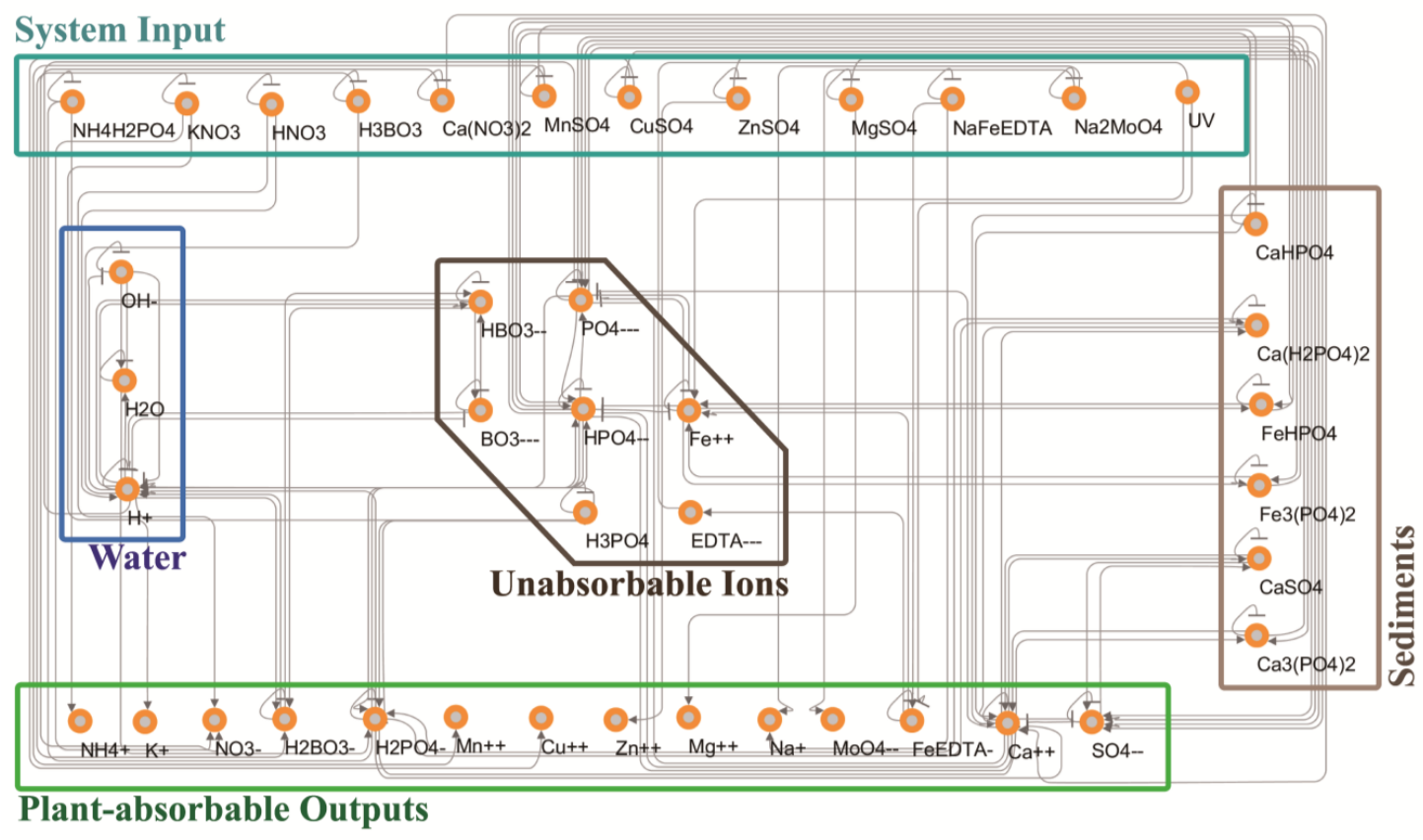
B. Network Dynamics Design
Reaction rate coefficients are driven from equilibrium constants by the relation K = kf/kb. Equilibrium constant is a description of a state of convergence so if we manipulate the value of kf and kb while fixing their ration as K, the reaction converges within the same status if time stride is not too big. Therefore, if we let kf = K and kb = 1 , the differential equation converges appropriately because their rate is still K, but the required time to make convergence only differs. It also can describe ionization and its reverse process, which are not actually chemical reactions.
We used dissociation constant Kd, which explains a reversible process in which big components breaks down into smaller components, to explain liquid state input such as nitric acid. For example, the equilibrium state of a reversible dissociation process XaYb ⇋aX+ bY is described as equation (2). Kd is directly obtain by gathering literature value of acid dissociation constant Ka. The solubility product equilibrium constant Ksp is adopted for dissolution of solids because it describes the dynamic equilibrium between solid and ion state. Solubility product equilibrium constant for dissolution Z(s) ⇋aX(aq) + bY(aq) is defined as equation (3), which is easily calculated with solubility.
Although simple application of kf and kb driven above can predict converged state of the system, it is not enough to describe system states before convergence. Therefore, we multiplied correction coefficient, which is a positive number between 1 and 1000, to correct the speed of forward and backward reactions. For example, dissociation of HNO3 into H+ and NO3- is very fast but dissolution of NaFe-EDTA into Na+ and Fe-EDTA- is relatively slow. So we multiplied 1000 to both kf and kb for nitric acid dissolution process and multiplied 1 to those of ferric EDTA.
Literature values of Ka, solubility for all reactions and calculated equilibrium constants involved in the experiments are provided on S2 in the supplementary information section. The differential equations, their reaction rate coefficients and correction coefficients used to perform simulations are listed in Table S3 on the supplementary information section.
III. Algorithm
The system needs initial state information. As the kinetics are time-dependent, the model is an ordinary differential equation model. An ODE model updates its next-step status by applying current-state information. Let [Xi] the concentration of i-th node variable of the network. It is a timedependent variable. In other word, [Xi] is a function of time. ODE for [Xi] is equation (4), where q is total number of terms in superpositioned equation for [Xi]. Coefficient c means the number of Xi in the term.
Update for [Xi] along time is performed with gradientdescent-like method as equation (5), where ∆t is the time interval. If the time interval is too small, the system converges too slowly but if it is too big, the system may not converge.
We applied synchronous update method, which update all X values from all X, because chemical reactions in one solution occurs simultaneously. We defined X(t) as a vector of concentration of the nodes and simply calculated dX(t) dt to obtain gradient vector. Synchronous update with vector-form is described in equation (6).
We built a chemical complex system solver with Python language. This simulator receives a text file containing differential equations of chemical reactions and reaction rate coefficient and automatically performs superposition for overlapped variables. The chemical topology is driven during text parsing process. It also performs both forward and backward simulations. We also wrote a text file which contains the topological and kinetic information of nutrient solution model. Both chemical complex system solver and nutrient system model information file are provided as an open sourced python package at the authors’ Github repository: https://github.com/needleworm/nutrient_solution.
IV. Experiment
To examine the performance of the simulator, we performed experiment on Yamazaki’s nutrient solution. As ISEs have error in complex chemical system due to the ion interference phenomenon, traditional methods to selectively readjust individual ions are not feasible. We compared ISEobserved ion concentration with the model’s prediction, as well as the literacy value
A. Equipments
Vernier’s Go Direct® ISE series, GDX-NO3, GDX-NH4, GDX-CA, GDX-K, are used to measure the concentration of ions. KNO3, Ca(NO3)2-4H2O, NH4H2PO4, MgSO4-7H2O are used to produce Yamazaki’s nutrient solution for lettuce. The simulation was performed on Intel’s I7-6850K with Python 3.6. 10 different settings of simulations were done at the same time as the CPU has 12 thread. Total simulation was done in less than 1 minute.
B. In-situ Conecntration Measurement
We prepared 100 times more concentrated version of Yamazaki’s nutrient solution for lettuce. It consisted of 0.4M of KNO3, 0.1M of Ca(NO3)2 and 0.05M of NH4H2PO4. Chemical compounds which are needed for other ions of Yamazaki’s nutrient solution were omitted in order to avoid any ions which are unmeasurable with our ISE devices.
By adding the concentrated solution on 1L water, we gradually increased the ionic concentration. Total 10 steps of addition was conducted and theoretical value for individual ions at each experimental step are provided on Table 1.
| 1 | 2 | 3 | 4 | 5 | 6 | 7 | 8 | 9 | 10 | |
|---|---|---|---|---|---|---|---|---|---|---|
| K | ||||||||||
| Theoretical Value | 3.8835 | 7.327 | 10.689 | 13.87 | 16.885 | 19.747 | 22.467 | 25.055 | 27.521 | 29.873 |
| Simulator Prediction | 3.8835 | 7.327 | 10.689 | 13.87 | 16.885 | 19.747 | 22.467 | 25.055 | 27.521 | 29.873 |
| Experimental Value | 4.36955 | 7.96121 | 11.3368 | 14.5715 | 17.55282 | 21.32524 | 24.19406 | 27.28197 | 30.85615 | 34.4981 |
| Ca | ||||||||||
| Theoretical Value | 0.97087 | 1.832 | 2.672 | 3.467 | 4.221 | 4.937 | 5.617 | 6.264 | 6.88 | 7.468 |
| Simulator Prediction | 0.97087 | 1.832 | 2.67199 | 3.46699 | 4.220957 | 4.936942 | 5.616895 | 6.263866 | 6.87983 | 7.4678 |
| Experimental Value | 0.95579 | 1.54849 | 2.04874 | 2.31673 | 2.650174 | 3.119853 | 3.356937 | 3.65157 | 3.790148 | 4.00463 |
| NO3 | ||||||||||
| Theoretical Value | 5.82524 | 10.991 | 16.033 | 20.804 | 25.327 | 26.92 | 33.7 | 37.582 | 41.281 | 44.81 |
| Simulator Prediction | 5.82524 | 10.991 | 16.033 | 20.804 | 25.327 | 29.621 | 33.701 | 37.583 | 41.281 | 44.809 |
| Experimental Value | 4.04472 | 8.24084 | 12.1232 | 16.0027 | 19.1123 | 22.95228 | 25.57974 | 29.36491 | 31.64328 | 34.8821 |
| NH4 | ||||||||||
| Theoretical Value | 0.48544 | 0.916 | 1.336 | 1.734 | 2.111 | 2.468 | 2.808 | 3.132 | 3.44 | 3.734 |
| Simulator Prediction | 0.48544 | 0.916 | 1.336 | 1.7339 | 2.111 | 2.468 | 2.808 | 3.132 | 3.44 | 3.734 |
| Experimental Value | 0.81084 | 1.46115 | 2.09361 | 2.68363 | 3.104724 | 3.616726 | 4.101231 | 4.388624 | 4.899455 | 5.34784 |
C. Simulation
The network model simulator was designed to receive various parameters: names of components, initial concentration, ionic state, reaction rate coefficient and the stirring velocity of water. We set the initial concentration values of KNO3, Ca(NO3)2 and NH4H2PO4 as the same value from wet experiment’s. And we set the initial value of any other components except H2O, H+ and OH- into 0 in order to make the simulation and experimental condition be same.
The time step dt was set to 1e-8 second to avoid stepupdate related issue. Although the concentration doesn’t show divergence, some ions with low concentration sometimes converged into wrong value when dt was set to 1e-4 second. The authors recommend using smaller time step for each update. Each simulation was terminated after 2.5 million updates, which took less than 50 seconds.
V. Result
The results from in-situ concentration measurement and simulation are provided on Table 1. The values are in mol per milliliter scale.
The simulator predicted theoretical value almost exactly. However, all the experimental value showed significant error. The error becomes greater at higher-concentration condition.
VI. Conclusion
Experiment showed that ion interference effect makes ISE value unclear. The errors of experimental values are not related to calibration or sensor malfunction because the ISE were calibrated with single-ion state solutions, whose concentration is exactly same as the solutions used for wet experiment. As interfering ions disturb Nernst potential on the membrane of ISE, any glass-based sensory device has ion interference issue. Therefore, applying ISEs on industrial condition to maintain nutrient solution is not feasible.
However, the network model provided in this paper has no prediction error even the prediction was gradient-descent based approach rather than calculation of dissociational value of chemical components directly. Applying complex system modeling would help removal of limitation of ISE approach and provide more precise status of nutrient solution system.
Acknowledgment
The authors would like to express our gratitude to Janghun Lee for development of ISE data acquisition software for sensory experiment.
This work was supported by the Technology Development Program S2679021 funded by the Ministry of SMEs and Startups (MSS, Korea).
Supplementary Informations
S1. Equations for simulation
S2. Ksp and Ka
S3. kf and kb
| Coefficient | Value | Coefficient | Value |
|---|---|---|---|
| k₀ | 1e-20 | k₁ | 1e-6 |
| k₂ | 976.8870716 | k₃ | 0 |
| k₄ | 161.1897361 | k₅ | 0 |
| k₆ | 105.7203812 | k₇ | 0 |
| k₈ | 0.725 | k₉ | 100 |
| k₁₀ | 6.31e-6 | k₁₁ | 100 |
| k₁₂ | 3.98e-13 | k₁₃ | 100 |
| k₁₄ | 1e-5 | k₁₅ | 100 |
| k₁₆ | 1.2e-16 | k₁₇ | 100 |
| k₁₈ | 0.591361 | k₁₉ | 100 |
References
-
[1] Cho W J, Kim H J, Jung D H, Kim D W, Ahn T I, Son J E. On-site ion monitoring system for precision hydroponic nutrient management. Comput Electron AGR. 2018; 146: 51-58. https://doi.org/10.1016/j.compag.2018.01.019.
-
[2] Bamsey M, Graham T, Thompson C, Berinstain A, Scott A, Dixon M. Ion-specific nutrient management in closed systems: the necessity for ion-selective sensors in terrestrial and space-based agriculture and water management systmes. Sensors. 2012; 12(10): 13349-13392. https://doi.org/10.3390/s121013349.
-
[3] Katsoulas N, Savvas D, Kitta E, Bartzanas T, Kittas C. Extension and evaluation of a model for automatic drainage solution management in tomato crops grown in semi-closed hydroponic systems. Comput Electron AGR. 2015; 113: 61-71. https://doi.org/10.1016/j.compag.2015.01.014.
-
[4] Ahn T I, Shin J W, Son J E, Analysis of Changes in Ion Concentration with Time and Drainage Ratio under EC-based Nutrient Control in Closed-loop Soilless Culture for Sweet Pepper Plants (Caspsicum Annum L. ‘Boogie’). J Bio-Environ Control. 2010; 19: 298-304.
-
[5] Neocleous D, Savvas D. NaCl accumulation and macroutrient uptake by a melon crop in a closed hydroponic system in relation to water uptake. Agric Water Manag. 2015; 165: 22-32. https://doi.org/10.1016/j.agwat.2015.11.013.
-
[6] Neocleous D, Savvas D. Simulating NaCl accumulation in a closed hydroponic crop of zucchini: Impact on macronutrient uptake, growth, ield, and photosynthesis. J Plant Nutr Soil SC. 2017; 180(3): 283-293. https://doi.org/10.1002/jpln.201600338.
-
[7] Kim H J, Son D W, Kwon S G, Roh M Y, Kang C I, Jung H S. PVC membrane-based portable ion analyzer for hydroponic and water monitoring. Comput Electron Agric. 2017; 140: 374-385. https://doi.org/10.1016/j.compag.2017.06.015.
-
[8] Ryan S Knight, Mark Lefsrud. Automated Nutrient Sensing and Recycling. 2017 ASABE Annual International Meeting. 2017; 1701609. https://doi.org/10.13031/aim.201701609.
-
[9] Jung D H, Kim H J, Kim W K, Kang C I, Choi G L. Automated Sensing and Control of Hydroponic Macronutrients Using a Computercontrolled System. ASABE. 2013; 131594020. https://doi.org/10.13031/aim.20131594020.
-
[10] Choi M, Shi J, Zhu Y, Yang R, Cho K H. Network dynamics-based cancer panel stratification for systemic prediction of anticancer drug response. Nat Commun. 2017; 8: 1940. https://doi.org/10.1038/s41467-017-02160-5
-
[11] Choo S M, Ban B, Joo J I, Cho K H. The phenotype control kernel of a biomolecular regulatory network. BMC Syst Biol. 2018; 12-49. https://doi.org/10.1186/s12918-018-0576-8
-
[12] Kim Y, Choi S, Shin D, Cho K H. Quantitative evaluation and reversion analysis of the attractor landscapes of an intracellular regulatory network for colorectal cancer. BMC syst boil. 2017; 11-45. https://doi.org/10.1186/s12918-017-0424-2
-
[13] Fumia H F, Martins M L. Boolean Network Model for Cancer Pathways: Predicting Carcinogenesis and Targeted Therapy Outcomes. PLoS One. 2013; 8(7). https://doi.org/10.1371/journal.pone.0069008
-
[14] Ban B, Kim S. Control of nonlinear, complex and black-boxed greenhouse system with reinforcement learning. 2017 ICTC; 2017 Oct 18-20; Jeju, South Korea; IEEE, 2017. https://doi.org/10.1109/ICTC.2017.8190813.
-
[15] Xu A M, Huang P H. Receptor Tyrosine Kinase Coactivation Network in Cancer. Cancer Res. 2010; 70(10): 3857-3860. https://doi.org/10.1158/0008-5472.CAN-10-0163.
-
[16] Grieco L, Calzone L, Bernard-Pierrot I, Radvanyi F, Kahn-Perles B, Thieffry D. Integrative Modeling of the Influence of MAPK Network on Cancer Cell Fate Decision. PLoS Comput Biol. 2013; 9(11): e1003286. https://doi.org/10.1371/journal.pcbi.1003286.
-
[17] Smith M C, Chao W, Kumar M, Francisco J S, Takahashi K, Lin J J. Temperature-Depentent Rate Coefficients for Reaction of CH2OO with Hydrogen Sulfide. J Phys Chem. 2017; 121 (5): 938-845. https://doi.org/10.1021/acs.jpca.6b12303.
-
[18] Raue A, Schilling M, Bachmann J, Matteson A, Schelker M, Kashchek D, et al. Lessons learnd from quantitative dynamical modeling in systems biology. PLoS One. 2013; 8: e74335.
-
[20] Frohlich F, Kessler T, Weindl D, Shadrin A, Schmiester L, Hache H, et al. Efficient Parameter Estimation Enables the Prediction of Drug Response Using a Mechanistic Pan-Cancer Pathway Model. Cell Syst. 2018; 7(6): 567-579. https://doi.org/10.1016/j.cels.2018.10.013.
-
[21] Yamazaki K. Nutrient solution culture. Tokyo, Japan: Pak-kyo Co; 1982. Japanese.
-
[22] Gao H, Mao H, Zhang X. Determination of lettuce nitrogen content using spectroscopy with efficient wavelength selection and extreme learning machine. Zemdirbyste. 2015; 102(1): 51-58. https://doi.org/10.13080/z-a.2015.102.006.
-
[23] Shannon P, Markei A, Ozier O, Baliga N S, Wang J T, Ramage D, et al. Cytoscape: a software environment for integrated models of biomolecular interaction networks. Genome Res. 2003; 13(11): 24982504. https://doi.org/10.1101/gr.1239303
-
[24] Lide, David R. CRC handbook of chemistry and physics: a readyreference book of chemical and physical data . CRC press, 1995.
-
[25] O'Neil, M.J. (ed.). The Merck Index - An Encyclopedia of Chemicals, Drugs, and Biologicals. Whitehouse Station, NJ: Merck and Co., Inc. ,2006., p. 1266
-
[26] Lide, D.R. (ed). CRC Handbook of Chemistry and Physics. 72nd ed. Boca Raton, FL: CRC Press, 1991-1992., p. 4-49
Citation
형식을 누르면 인용 정보가 복사됩니다.